Skip to content

Chapter 26

Optimal and adaptive filtering

Four lessons in Part IX, Random signals and statistical signal processing. Read them in order, or start anywhere: a prerequisite is a link, never a gate.

Start with 26.1
0 of 4 read1 on the essential pathabout 80 minutes

Lessons in this chapter

Two stacked panels. Received x[n]: 512 noisy samples, n = 0 to 511, with the 64-sample template drawn over them at the current lag and a bracket marking it. Matched-filter output: the sum of the products at each lag ℓ, from 0 to 448. Lag ℓ = 448: the template covers samples 448 to 511, and the output there is −6.7; the output is drawn for lags 0 to 448. A diamond marks the peak, 31.8 at lag 300.Two stacked panels. Received x[n]: 512 noisy samples, n = 0 to 511, with the 64-sample template drawn over them at the current lag and a bracket marking it. Matched-filter output: the sum of the products at each lag ℓ, from 0 to 448. Lag ℓ = 448: the template covers samples 448 to 511, and the output there is −6.7; the output is drawn for lags 0 to 448. A diamond marks the peak, 31.8 at lag 300.

Lesson 1 Essential16 minYou are hereRead

Matched filters and detection

To find a known pulse in white noise, correlate with it: no linear filter lifts it further above the noise. A threshold then decides.

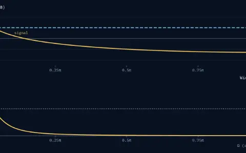
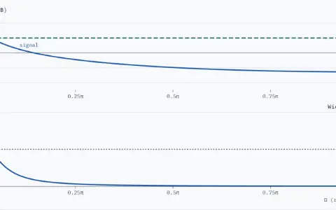
Two stacked panels against Ω from 0 to π. PSDs, in dB from −25 to 25: the signal's PSD, a solid curve labelled signal, from 12.8 dB at 0 to −12.8 dB at π, and the noise's PSD, a flat dashed line labelled noise. Wiener gain H_opt, from 0 to 1, with a dotted level at ½. Noise at 10 dB. The gain is 0.655 at 0 and 0.005 at π, ½ at 0.032π, where a small tick marks it. Error power 0.586.Two stacked panels against Ω from 0 to π. PSDs, in dB from −25 to 25: the signal's PSD, a solid curve labelled signal, from 12.8 dB at 0 to −12.8 dB at π, and the noise's PSD, a flat dashed line labelled noise. Wiener gain H_opt, from 0 to 1, with a dotted level at ½. Noise at 10 dB. The gain is 0.655 at 0 and 0.005 at π, ½ at 0.032π, where a small tick marks it. Error power 0.586.

Lesson 220 minYou are hereRead

The Wiener filter

Recover a signal from noise with the least mean-square error: weight each frequency by the signal's share of the power, or solve the Wiener–Hopf equations.

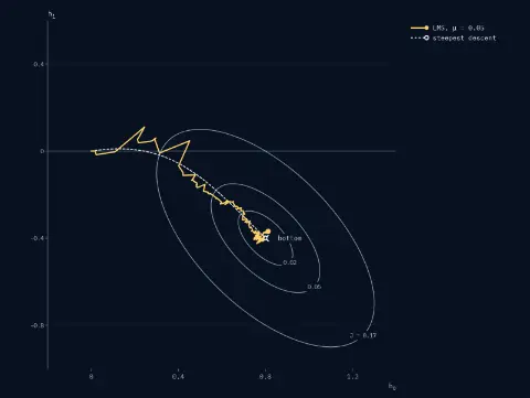
One panel, the two taps at equal scales: h_0 across from −0.2 to 1.4, h_1 up from −1.0 to 0.6. Contours of the error J at 0.02, 0.05, 0.17: ellipses around the bottom, h_true = (0.800, −0.400), marked by a cross. The steepest-descent path is dashed; the LMS path is solid, with a mark at the current taps. Step size μ = 0.05. After 300 steps, LMS is at (0.812, −0.369), J = 0.012; steepest descent at (0.799, −0.399), J = 0.010.One panel, the two taps at equal scales: h_0 across from −0.2 to 1.4, h_1 up from −1.0 to 0.6. Contours of the error J at 0.02, 0.05, 0.17: ellipses around the bottom, h_true = (0.800, −0.400), marked by a cross. The steepest-descent path is dashed; the LMS path is solid, with a mark at the current taps. Step size μ = 0.05. After 300 steps, LMS is at (0.812, −0.369), J = 0.012; steepest descent at (0.799, −0.399), J = 0.010.

Lesson 322 minYou are hereRead

Adaptive filters: LMS

A filter that learns its taps: LMS walks down the error bowl in noisy steps, and an adaptive canceller removes mains hum.

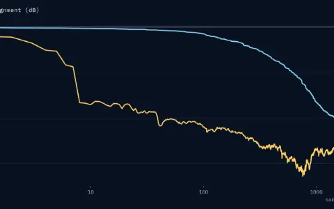
Misalignment in dB against sample n from 1 to 2000 on a logarithmic axis, for LMS (a line ending in a square) and RLS (a line ending in a dot), identifying 8 taps from a coloured input. Both curves drawn up to sample 2000: LMS at −47.1 dB, RLS at −56.1 dB.Misalignment in dB against sample n from 1 to 2000 on a logarithmic axis, for LMS (a line ending in a square) and RLS (a line ending in a dot), identifying 8 taps from a coloured input. Both curves drawn up to sample 2000: LMS at −47.1 dB, RLS at −56.1 dB.

Lesson 422 minYou are hereRead

RLS and the Kalman filter

RLS solves least squares again at every sample, so it learns fast; the Kalman filter predicts with a model and corrects with measurements.

After this chapter

Where to go next.

The chapters either side, and the rest of Part IX in the library.

Phasorium
LibraryEvery lesson, in order

Parts

About Phasorium
Look