Skip to content

Chapter 25

Spectral estimation

Four lessons in Part IX, Random signals and statistical signal processing. Read them in order, or start anywhere: a prerequisite is a link, never a gate.

Start with 25.1
0 of 4 read2 on the essential pathabout 78 minutes

Lessons in this chapter

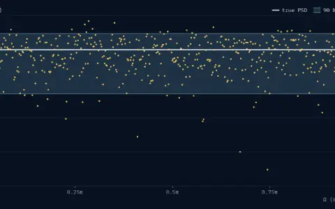
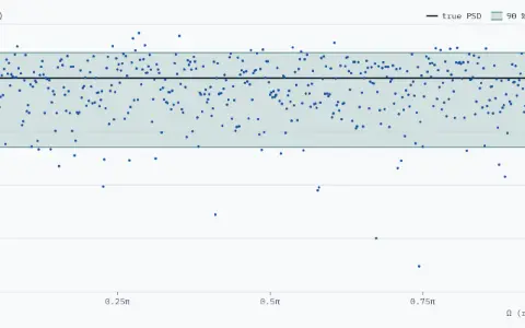
Periodogram of the first 1024 samples of white Gaussian noise: 511 dots, one per bin, from −35.2 dB to 8.4 dB. A shaded band, 90 % of values, runs from −12.9 dB to 4.8 dB, and a solid line marks the true PSD at 0 dB; 462 of the 511 dots lie in the band. Mean 1.025, spread ÷ mean 0.963.Periodogram of the first 1024 samples of white Gaussian noise: 511 dots, one per bin, from −35.2 dB to 8.4 dB. A shaded band, 90 % of values, runs from −12.9 dB to 4.8 dB, and a solid line marks the true PSD at 0 dB; 462 of the 511 dots lie in the band. Mean 1.025, spread ÷ mean 0.963.

Lesson 1 Essential18 minYou are hereRead

The periodogram

Square a record's DFT and divide by N: the obvious PSD estimate. It scatters as widely at any length, and short records blur its peaks.

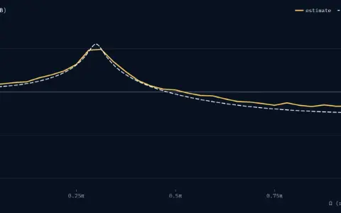
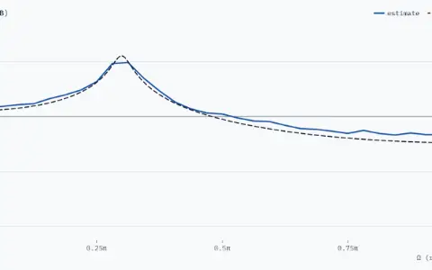
One panel, PSD in dB against Ω from 0 to π: the true PSD of the AR(2) noise as a dashed line, peaking at 22.1 dB near Ω = 0.3π, and the estimate as a solid line. Segment length L = 64: K = 64 segments, spread 0.50 dB, average peak 20.6 dB.One panel, PSD in dB against Ω from 0 to π: the true PSD of the AR(2) noise as a dashed line, peaking at 22.1 dB near Ω = 0.3π, and the estimate as a solid line. Segment length L = 64: K = 64 segments, spread 0.50 dB, average peak 20.6 dB.

Lesson 2 Essential18 minYou are hereRead

Averaged periodograms: Bartlett and Welch

Cut one record into segments and average their periodograms: the scatter shrinks, the peaks blur, and overlapping Hann-windowed segments buy extra averages.

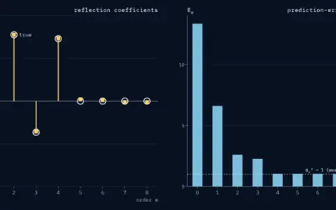
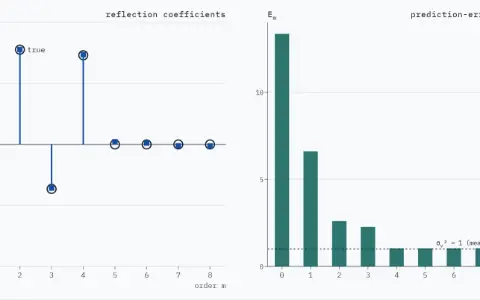
Two panels. Reflection coefficients k_m for orders 1 to 8: estimates as stems with square heads, the true values as open rings marked true (−0.714, 0.777, −0.364, 0.731, 0.000, 0.000, 0.000, 0.000). Prediction-error power E_m for orders 0 to 8 as bars, with a dotted level at σ_v² = 1, measured 1.003. Orders 1 to 8 computed: k = −0.711, 0.778, −0.358, 0.736, 0.022, 0.011, −0.011, −0.012; E falls from 13.350 to 1.040.Two panels. Reflection coefficients k_m for orders 1 to 8: estimates as stems with square heads, the true values as open rings marked true (−0.714, 0.777, −0.364, 0.731, 0.000, 0.000, 0.000, 0.000). Prediction-error power E_m for orders 0 to 8 as bars, with a dotted level at σ_v² = 1, measured 1.003. Orders 1 to 8 computed: k = −0.711, 0.778, −0.358, 0.736, 0.022, 0.011, −0.011, −0.012; E falls from 13.350 to 1.040.

Lesson 322 minYou are hereRead

Parametric models and linear prediction

Fit a few coefficients instead of estimating every bin: predict each sample from its past, solve Yule–Walker order by order, and read a smooth spectrum.

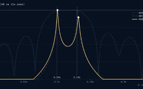
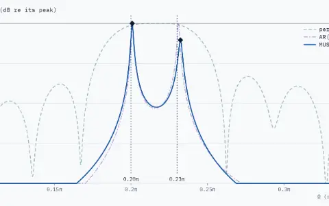
Three spectral estimates of 64 samples of two tones in noise, each in dB re its own peak, for Ω from 0.1π to 0.35π; values below −40 dB are drawn on the floor. Dotted vertical lines mark the true tones at 0.20π and 0.23π. Solid line: MUSIC, 2 peaks, diamonds at 0.201π and 0.232π. Faint dashed line: the periodogram and faint dash-dot line: Burg's AR(16).Three spectral estimates of 64 samples of two tones in noise, each in dB re its own peak, for Ω from 0.1π to 0.35π; values below −40 dB are drawn on the floor. Dotted vertical lines mark the true tones at 0.20π and 0.23π. Solid line: MUSIC, 2 peaks, diamonds at 0.201π and 0.232π. Faint dashed line: the periodogram and faint dash-dot line: Burg's AR(16).

Lesson 420 minYou are hereRead

High-resolution frequency estimation

Two tones closer than one bin blur into one periodogram lump; Burg's AR model and MUSIC, which uses eigenvectors, split them.

Phasorium
LibraryEvery lesson, in order

Parts

About Phasorium
Look