Probability

Random variables

A random variable attaches a number to each outcome, and its distribution says how likely each value is. This topic computes expected values and variances, moves from counts to densities, meets the normal distribution, and transforms one random variable into another.

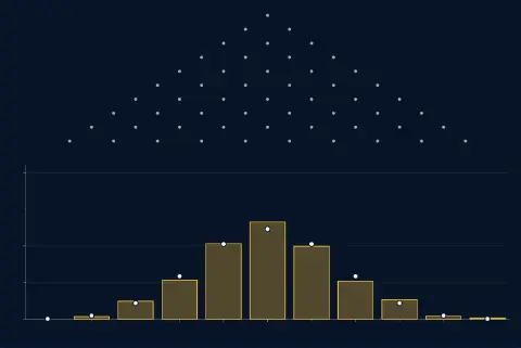
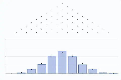
A board of 10 rows of pegs above 11 bins for 0 to 10 rights; each ball goes right at a peg with chance 0.50. 1000 balls have landed; the bars show their shares: 0.000, 0.007, 0.049, 0.106, 0.206, 0.265, 0.199, 0.104, 0.053, 0.008, 0.003. A dot on each bin marks the long-run share: 0.0010, 0.0098, 0.0439, 0.1172, 0.2051, 0.2461, 0.2051, 0.1172, 0.0439, 0.0098, 0.0010.

A board of 10 rows of pegs above 11 bins for 0 to 10 rights; each ball goes right at a peg with chance 0.50. 1000 balls have landed; the bars show their shares: 0.000, 0.007, 0.049, 0.106, 0.206, 0.265, 0.199, 0.104, 0.053, 0.008, 0.003. A dot on each bin marks the long-run share: 0.0010, 0.0098, 0.0439, 0.1172, 0.2051, 0.2461, 0.2051, 0.1172, 0.0439, 0.0098, 0.0010.

Beginner · 30 minYou are hereRead

Discrete random variables

A random variable attaches a number to each outcome; its probability mass function says how likely each is, and falling balls draw it.

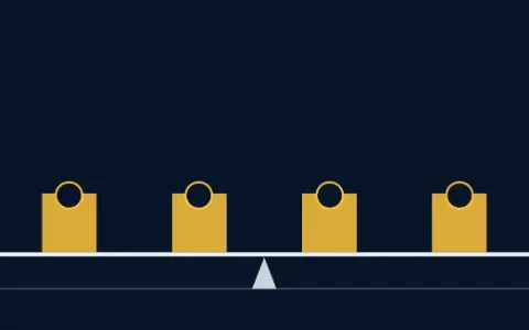
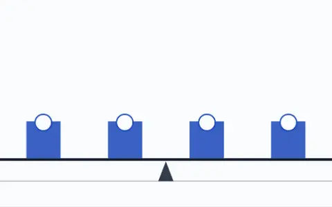
A beam marked 1 to 6 carries six bars of heights 0.17, 0.17, 0.17, 0.17, 0.17, 0.17, over a triangle pivot at 3.50. The beam is level.

A beam marked 1 to 6 carries six bars of heights 0.17, 0.17, 0.17, 0.17, 0.17, 0.17, over a triangle pivot at 3.50. The beam is level.

Intermediate · 30 minYou are hereRead

Expected value

The mean is the probability-weighted average of a random variable, and the point where its distribution balances like weights on a beam.

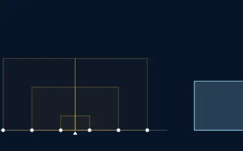
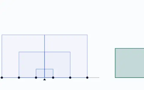
A number line from 0.5 to 6.5 with six dots at 1.00, 2.00, 3.00, 4.00, 5.00, 6.00, each with chance 1/6, and the mean 3.50 marked. Squares from the dots out to the mean, of areas 6.25, 2.25, 0.25, 0.25, 2.25, 6.25. Beside them, their average: a square of area 2.9167 and side 1.7078.

A number line from 0.5 to 6.5 with six dots at 1.00, 2.00, 3.00, 4.00, 5.00, 6.00, each with chance 1/6, and the mean 3.50 marked. Squares from the dots out to the mean, of areas 6.25, 2.25, 0.25, 0.25, 2.25, 6.25. Beside them, their average: a square of area 2.9167 and side 1.7078.

Intermediate · 30 minYou are hereRead

Variance and standard deviation

Spread is the average squared distance from the mean, drawn as squares; its square root, the standard deviation, is in the units of the data.

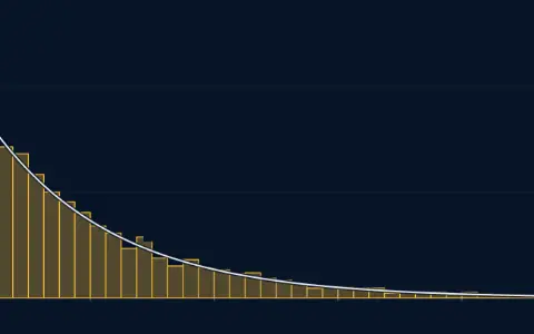
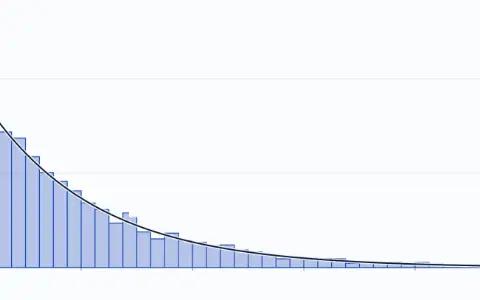
Histogram of 5000 draws from the exponential law in 40 bins 0.125 wide from 0 to 5, each bar count over draws times width; the tallest bar is 0.880. The curve e^(−x), labelled exact density, is drawn over the bars. The bars' area is 0.994.

Histogram of 5000 draws from the exponential law in 40 bins 0.125 wide from 0 to 5, each bar count over draws times width; the tallest bar is 0.880. The curve e^(−x), labelled exact density, is drawn over the bars. The bars' area is 0.994.

Intermediate · 30 minYou are hereRead

Continuous random variables

A density gives probability as area under a curve, so any single exact value has probability zero, and a density can rise above 1.

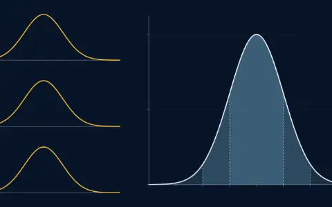
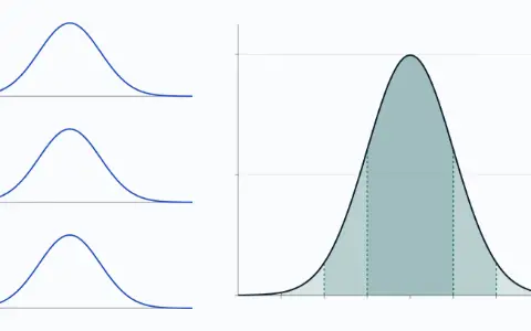
Three bells, for adult heights, exam scores and radio noise, each now the standard bell on an axis of z from −4 to 4. Below, the standard bell. Shaded bands: within 1, 68.27 %; within 2, 95.45 %; within 3, 99.73 %.

Three bells, for adult heights, exam scores and radio noise, each now the standard bell on an axis of z from −4 to 4. Below, the standard bell. Shaded bands: within 1, 68.27 %; within 2, 95.45 %; within 3, 99.73 %.

Intermediate · 30 minYou are hereRead

The normal distribution

Every bell curve is one bell stretched and shifted, so one set of areas serves them all, as long as the data really are bell-shaped.

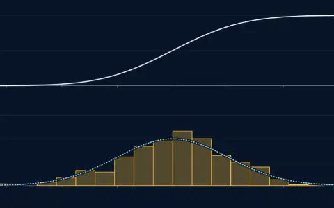
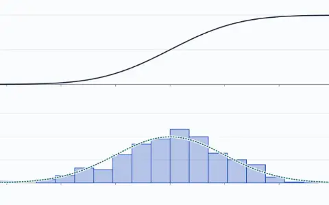
Top, the standard normal distribution function F rising from 0 to 1 against x from −3.50 to 3.50; heights u on the left axis. Below, a histogram of the 400 values landed so far. The standard normal density is outlined over it.

Top, the standard normal distribution function F rising from 0 to 1 against x from −3.50 to 3.50; heights u on the left axis. Below, a histogram of the 400 values landed so far. The standard normal density is outlined over it.

Advanced · 30 minYou are hereRead

Transforming random variables

The density of a function of a random variable stretches with the map, and the inverse distribution function turns even dots into any shape.

Related topics

Where to go next.